Content Overview
Introduction
A national omnichannel retailer in India came to Codelynks with a specific problem: their “real-time inventory” system was 47 minutes stale at peak, which meant their BOPIS (buy online, pick up in store) promise was failing one in four customers during sale events. They had Apache Kafka feeding a mature data warehouse. They had a data engineering team that understood both tools. The problem was not their tooling. The problem was that they had built a streaming ingestion layer on top of a batch table format, and the two had incompatible consistency models.
The inventory data was arriving continuously via Kafka. The warehouse was processing it in micro-batches every 90 seconds. During peak transaction hours, warehouse file compaction paused to handle query load, micro-batches accumulated in the staging layer, and inventory data fell 30 to 50 minutes behind. Adding more Kafka consumers made it worse. Every additional consumer increased write volume on the warehouse, which extended compaction time, which increased the lag.
This is the pattern we see in retail data platforms that were designed before Apache Iceberg became operational. The 2026 architecture question is no longer whether to adopt Iceberg. It is how to run it as a production product at retail transaction volumes without recreating the same bottleneck.
Why Real-Time Inventory Fails Before You Add More Kafka Workers
Batch ETL pipelines were designed for end-of-day inventory reconciliation. When retail moved to omnichannel with POS systems, warehouse management, e-commerce, and marketplace feeds all updating inventory simultaneously the batch model was stretched past its operating range without a fundamental architecture change.
The write amplification problem: every small write to a data warehouse creates a new file. At 10,000 POS transactions per hour across 200 stores, that is a continuous stream of small files landing in the storage layer. Traditional data warehouses and first-generation data lakes handle this by compacting files in background jobs that consolidate many small files into fewer large ones. When compaction is running, query performance degrades. When query load spikes (during a sale), compaction is deprioritized, files accumulate, and read performance worsens. The cycle repeats.
Apache Iceberg breaks this cycle at the format level. Iceberg tables use a metadata layer that tracks file-level statistics, partition snapshots, and row-level deletes without rewriting entire files. A write to an Iceberg table creates a new snapshot that references changed files it does not invalidate existing query plans. This means concurrent reads and writes do not compete in the same way they do on a traditional warehouse table. Deletion vectors (introduced in Iceberg v3, now in public preview on Databricks as of May 2026) extend this to row-level updates: a position delete can be applied without a full file rewrite.
Your inventory data is 47 minutes stale not because you lack Kafka workers, but because your table format was designed for nightly batch loads.
What Apache Iceberg v3 Changes for Retail Data Teams
Databricks released Apache Iceberg v3 to public preview in May 2026. Three features matter specifically for retail inventory architecture.
Deletion vectors at scale: Previous Iceberg versions handled row deletes via position delete files, which required merge-on-read at query time for high-delete-rate tables. V3 deletion vectors batch these efficiently, reducing the merge-on-read overhead for tables that receive continuous CDC (change data capture) updates. For a retail inventory table with thousands of position updates per minute, this changes the cost model for real-time ingestion.
Row lineage: Iceberg v3 tracks the origin of every row through insert, update, and delete operations. For a retailer running BOPIS and ship-from-store, this enables exact inventory attribution when an item is reserved, deducted, restocked, or returned, the full lineage is queryable without a separate audit table.
Improved manifest handling for high-partition tables: Retail inventory tables are typically partitioned by store ID, SKU category, and date. At 5,000 stores and 200,000 SKUs, partition count is high. V3 manifest improvements reduce the metadata scan cost for queries against recent partitions, which is where inventory freshness queries always land.
None of these features eliminate the need for compaction. They reduce the frequency and cost of compaction relative to previous Iceberg versions and relative to traditional warehouse formats.
The Retail Data Freshness Ladder (RDFL)
The RDFL is a four-tier framework for measuring and targeting inventory data latency across retail data platforms. Each tier has a technical definition, a business implication, and an architecture requirement.
Tier 1: Batch (Latency: 4 to 24 hours)
Data arrives via nightly ETL from ERP, WMS, and POS systems. Appropriate for financial reconciliation, vendor purchase order generation, and historical analytics. Insufficient for any customer-facing inventory display. Architecture: standard data warehouse, no streaming.
Tier 2: Near Real-Time (Latency: 5 to 30 minutes)
Micro-batch ingestion from core systems. Data is fresh enough for replenishment triggers and back-office dashboards. Not reliable for BOPIS promise fulfillment during peak events. Architecture: streaming pipeline feeding a warehouse with micro-batch load intervals. This is where most omnichannel retailers sit today.
Tier 3: Operational Real-Time (Latency: 30 seconds to 5 minutes)
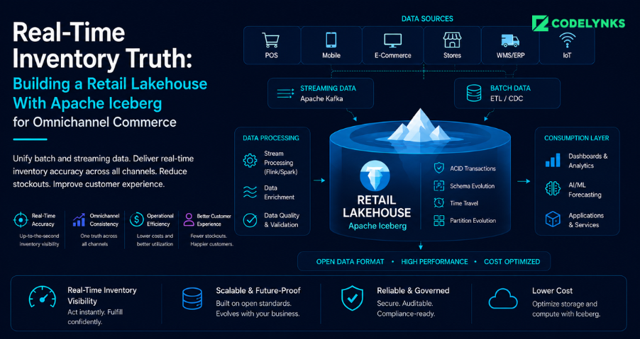
CDC-based ingestion from POS, WMS, and e-commerce via Kafka into Iceberg tables with frequent small-file compaction. Meets the latency requirement for BOPIS promise fulfillment and omnichannel inventory display. Architecture: Kafka + CDC connectors (Debezium) feeding Iceberg tables via a streaming SQL engine (Flink or Spark Structured Streaming), with a REST Catalog for query engine access.
Tier 4: Sub-Second Inventory (Latency: under 5 seconds)
Required only for high-velocity SKUs during flash sale events. Typically achieved by running a Redis or DynamoDB materialized view for hot SKUs alongside the Iceberg lakehouse for cold catalog. Architecture: dual-tier with cache invalidation driven by Kafka events and Iceberg as the source of truth for reconciliation.
Most national omnichannel retailers need Tier 3 for their BOPIS and omnichannel use cases. Tier 4 is a specialized layer for peak event handling, not a general architecture.
The retailer we worked with was operating at Tier 2 and needed Tier 3. The migration required three changes: replacing their micro-batch loader with Flink-based CDC ingestion, converting their inventory tables from Parquet-on-S3 to Iceberg format (a one-time migration that took 6 days for 18 months of history), and deploying a REST Catalog to unify access across their BI queries (Trino), ML pipelines (Spark), and operational dashboards (DuckDB via their internal API).
For teams evaluating data architecture options for retail platforms, see our [data engineering practice overview](/services/data-engineering) for how we approach lakehouse migrations.
The Architecture That Resolves Write Amplification
A national omnichannel retailer in India came to Codelynks with a specific problem: their “real-time inventory” system was 47 minutes stale at peak, which meant their BOPIS (buy online, pick up in store) promise was failing one in four customers during sale events. They had Apache Kafka feeding a mature data warehouse. They had a data engineering team that understood both tools. The problem was not their tooling. The problem was that they had built a streaming ingestion layer on top of a batch table format, and the two had incompatible consistency models.
The inventory data was arriving continuously via Kafka. The warehouse was processing it in micro-batches every 90 seconds. During peak transaction hours, warehouse file compaction paused to handle query load, micro-batches accumulated in the staging layer, and inventory data fell 30 to 50 minutes behind. Adding more Kafka consumers made it worse. Every additional consumer increased write volume on the warehouse, which extended compaction time, which increased the lag.
This is the pattern we see in retail data platforms that were designed before Apache Iceberg became operational. The 2026 architecture question is no longer whether to adopt Iceberg. It is how to run it as a production product at retail transaction volumes without recreating the same bottleneck.
Why Real-Time Inventory Fails Before You Add More Kafka Workers
Batch ETL pipelines were designed for end-of-day inventory reconciliation. When retail moved to omnichannel with POS systems, warehouse management, e-commerce, and marketplace feeds all updating inventory simultaneously the batch model was stretched past its operating range without a fundamental architecture change.
The write amplification problem: every small write to a data warehouse creates a new file. At 10,000 POS transactions per hour across 200 stores, that is a continuous stream of small files landing in the storage layer. Traditional data warehouses and first-generation data lakes handle this by compacting files in background jobs that consolidate many small files into fewer large ones. When compaction is running, query performance degrades. When query load spikes (during a sale), compaction is deprioritized, files accumulate, and read performance worsens. The cycle repeats.
Apache Iceberg breaks this cycle at the format level. Iceberg tables use a metadata layer that tracks file-level statistics, partition snapshots, and row-level deletes without rewriting entire files. A write to an Iceberg table creates a new snapshot that references changed files; it does not invalidate existing query plans. This means concurrent reads and writes do not compete in the same way they do on a traditional warehouse table. Deletion vectors (introduced in Iceberg v3, now in public preview on Databricks as of May 2026) extend this to row-level updates: a position delete can be applied without a full file rewrite.
Your inventory data is 47 minutes stale not because you lack Kafka workers, but because your table format was designed for nightly batch loads.
What Apache Iceberg v3 Changes for Retail Data Teams
Databricks released Apache Iceberg v3 to public preview in May 2026. Three features matter specifically for retail inventory architecture.
Deletion vectors at scale: Previous Iceberg versions handled row deletes via position delete files, which required merge-on-read at query time for high-delete-rate tables. V3 deletion vectors batch these efficiently, reducing the merge-on-read overhead for tables that receive continuous CDC (change data capture) updates. For a retail inventory table with thousands of position updates per minute, this changes the cost model for real-time ingestion.
Row lineage: Iceberg v3 tracks the origin of every row through insert, update, and delete operations. For a retailer running BOPIS and ship-from-store, this enables exact inventory attribution when an item is reserved, deducted, restocked, or returned, the full lineage is queryable without a separate audit table.
Improved manifest handling for high-partition tables: Retail inventory tables are typically partitioned by store ID, SKU category, and date. At 5,000 stores and 200,000 SKUs, partition count is high. V3 manifest improvements reduce the metadata scan cost for queries against recent partitions, which is where inventory freshness queries always land.
None of these features eliminate the need for compaction. They reduce the frequency and cost of compaction relative to previous Iceberg versions and relative to traditional warehouse formats.
The Retail Data Freshness Ladder (RDFL)
The RDFL is a four-tier framework for measuring and targeting inventory data latency across retail data platforms. Each tier has a technical definition, a business implication, and an architecture requirement.
Tier 1: Batch (Latency: 4 to 24 hours)
Data arrives via nightly ETL from ERP, WMS, and POS systems. Appropriate for financial reconciliation, vendor purchase order generation, and historical analytics. Insufficient for any customer-facing inventory display. Architecture: standard data warehouse, no streaming.
Tier 2: Near Real-Time (Latency: 5 to 30 minutes)
Micro-batch ingestion from core systems. Data is fresh enough for replenishment triggers and back-office dashboards. Not reliable for BOPIS promise fulfillment during peak events. Architecture: streaming pipeline feeding a warehouse with micro-batch load intervals. This is where most omnichannel retailers sit today.
Tier 3: Operational Real-Time (Latency: 30 seconds to 5 minutes)
CDC-based ingestion from POS, WMS, and e-commerce via Kafka into Iceberg tables with frequent small-file compaction. Meets the latency requirement for BOPIS promise fulfillment and omnichannel inventory display. Architecture: Kafka + CDC connectors (Debezium) feeding Iceberg tables via a streaming SQL engine (Flink or Spark Structured Streaming), with a REST Catalog for query engine access.
Tier 4: Sub-Second Inventory (Latency: under 5 seconds)
Required only for high-velocity SKUs during flash sale events. Typically achieved by running a Redis or DynamoDB materialized view for hot SKUs alongside the Iceberg lakehouse for cold catalog. Architecture: dual-tier with cache invalidation driven by Kafka events and Iceberg as the source of truth for reconciliation.
Most national omnichannel retailers need Tier 3 for their BOPIS and omnichannel use cases. Tier 4 is a specialized layer for peak event handling, not a general architecture.
The retailer we worked with was operating at Tier 2 and needed Tier 3. The migration required three changes: replacing their micro-batch loader with Flink-based CDC ingestion, converting their inventory tables from Parquet-on-S3 to Iceberg format (a one-time migration that took 6 days for 18 months of history), and deploying a REST Catalog to unify access across their BI queries (Trino), ML pipelines (Spark), and operational dashboards (DuckDB via their internal API).
The Architecture That Resolves Write Amplification
The core architecture for Tier 3 retail inventory:
The CDC connector (Debezium) reads the POS database binlog and WMS transaction log and publishes events to Kafka topics partitioned by store ID. A Flink job consumes these events, applies deduplication (a POS system may emit the same transaction event twice during a network retry), and writes directly to Iceberg tables using the Flink-Iceberg connector.
The Iceberg table for inventory positions uses a schema designed for CDC: the primary key is (store_id, sku_id), and the table uses merge-on-read semantics so that updates do not require rewriting the entire partition file. A compaction job runs on a 10-minute schedule outside of peak query windows, consolidating small files and cleaning deletion vectors.
A REST Catalog (Apache Polaris or managed equivalents on Databricks Unity Catalog or AWS Glue) provides a single governance layer. Every query engine Trino for BI queries, Spark for ML training pipelines, and the application API for real-time inventory checks reads from the same Iceberg metadata. Access controls are enforced at the catalog layer, not replicated across engines.
Compaction is the tax you pay for real-time writes. The teams that plan for it ship. The teams that discover it in production rebuild.
Operational Realities: Compaction, Catalog Governance, and the Multi-Engine Tax
The hardest part of running Iceberg at retail scale is not turning it on. It is running ingestion and compaction as a managed product.
Compaction must be scheduled, not run on-demand. A compaction job that kicks off during peak query hours degrades read performance. Most teams learn this at 3 a.m. on the day after their first sale event, when compaction from the sale’s write volume collides with the next morning’s BI jobs.
The multi-engine lakehouse where Flink, Trino, DuckDB, and Spark all read the same Iceberg tables requires centralized governance. Without a REST Catalog with role-based access control, each engine maintains its own metadata cache, which diverges under concurrent writes. The REST Catalog serializes metadata access and ensures every engine sees a consistent snapshot.
The counterintuitive number from the retailer engagement: migrating to Iceberg reduced their total storage cost by 31% within 90 days because Iceberg’s partition pruning eliminated the full-scan queries that were driving object storage egress charges. The real-time improvement was the headline goal. The storage savings paid for the migration.
What This Means for Retail and E-commerce Leaders
If your BOPIS cancel rate spikes during sale events, or if your inventory display accuracy drops below 95% during peak traffic, the architecture fix is almost certainly a move from Tier 2 to Tier 3 on the RDFL. The migration path is documented, the tooling is production-grade, and the operational requirements are understood.
Three steps you can take this week:
1. Measure your actual inventory data latency at peak. Not the theoretical pipeline interval the measured staleness between a POS transaction and the moment the inventory count changes in your e-commerce system. If you do not have this measurement, instrument it before any architecture discussion.
2. Ask your data engineering team whether your current inventory tables are stored in Iceberg, Delta Lake, Hudi, or a traditional Parquet-based warehouse format. If the answer is the latter, that is your write amplification source.
3. Check whether your compaction jobs have a scheduled window that does not overlap with your peak query hours. Most teams have compaction running as a continuous background process which means it always runs during peak.
The tooling is not the obstacle. Apache Iceberg is free, the Flink connector is production-grade, and REST Catalog is available as a managed service on every major cloud. The obstacle is building compaction and catalog governance as a product, not an afterthought.
CDC connector (Debezium) reads the POS database binlog and WMS transaction log and publishes events to Kafka topics partitioned by store ID. A Flink job consumes these events, applies deduplication (a POS system may emit the same transaction event twice during a network retry), and writes directly to Iceberg tables using the Flink-Iceberg connector.
The Iceberg table for inventory positions uses a schema designed for CDC: the primary key is (store_id, sku_id), and the table uses merge-on-read semantics so that updates do not require rewriting the entire partition file. A compaction job runs on a 10-minute schedule outside of peak query windows, consolidating small files and cleaning deletion vectors.
A REST catalog (Apache Polaris or managed equivalents on Databricks Unity Catalog or AWS Glue) provides a single governance layer. Every query engine, Trino for BI queries, Spark for ML training pipelines, and the application API for real-time inventory checks, reads from the same Iceberg metadata. Access controls are enforced at the catalog layer, not replicated across engines.
Compaction is the tax you pay for real-time writes. The teams that plan for it ship. The teams that discover it in production rebuild.
Operational Realities: Compaction, Catalog Governance, and the Multi-Engine Tax
The hardest part of running Iceberg at retail scale is not turning it on. It is running ingestion and compaction as a managed product.
Compaction must be scheduled, not run on-demand. A compaction job that kicks off during peak query hours degrades read performance. Most teams learn this at 3 a.m. on the day after their first sale event, when compaction from the sale’s write volume collides with the next morning’s BI jobs.
The multi-engine lakehouse where Flink, Trino, DuckDB, and Spark all read the same Iceberg tables requires centralized governance. Without a REST Catalog with role-based access control, each engine maintains its own metadata cache, which diverges under concurrent writes. The REST Catalog serializes metadata access and ensures every engine sees a consistent snapshot.
The counterintuitive number from the retailer engagement: migrating to Iceberg reduced their total storage cost by 31% within 90 days because Iceberg’s partition pruning eliminated the full-scan queries that were driving object storage egress charges. The real-time improvement was the headline goal. The storage savings paid for the migration.
What This Means for Retail and E-commerce Leaders
If your BOPIS cancel rate spikes during sale events, or if your inventory display accuracy drops below 95% during peak traffic, the architecture fix is almost certainly a move from Tier 2 to Tier 3 on the RDFL. The migration path is documented, the tooling is production-grade, and the operational requirements are understood.
Three steps you can take this week:
1. Measure your actual inventory data latency at peak. Not the theoretical pipeline interval the measured staleness between a POS transaction and the moment the inventory count changes in your e-commerce system. If you do not have this measurement, instrument it before any architecture discussion.
2. Ask your data engineering team whether your current inventory tables are stored in Iceberg, Delta Lake, Hudi, or a traditional Parquet-based warehouse format. If the answer is the latter, that is your write amplification source.
3. Check whether your compaction jobs have a scheduled window that does not overlap with your peak query hours. Most teams have compaction running as a continuous background process which means it always runs during peak.
The tooling is not the obstacle. Apache Iceberg is free, the Flink connector is production-grade, and REST Catalog is available as a managed service on every major cloud. The obstacle is building compaction and catalog governance as a product, not an afterthought.
About the author: The Codelynks data engineering team designs and migrates retail data platforms for omnichannel operators across India and Southeast Asia. [Connect on LinkedIn](https://www.linkedin.com/company/codelynks).*
FAQ’s
Apache Iceberg is an open table format for large-scale analytical datasets. Unlike traditional Parquet-based warehouse tables, Iceberg uses a metadata layer that enables ACID-compliant transactions, concurrent reads and writes without conflicts, and efficient row-level updates. For retail inventory data that changes continuously across POS, WMS, and e-commerce systems, these properties reduce data staleness from minutes to seconds.
Write amplification occurs when a streaming workload generates more write operations than the underlying storage format can compact efficiently. In retail, high-frequency POS and WMS events create many small files. When the system cannot compact these files fast enough, read queries slow down and inventory latency increases. Apache Iceberg’s deletion vectors and snapshot isolation architecture reduce write amplification compared to traditional warehouse formats.
The RDFL is a four-tier framework developed by Codelynks for measuring and targeting inventory data latency. Tier 1 is batch (4 to 24 hours), appropriate for financial reconciliation. Tier 2 is near real-time (5 to 30 minutes), common in most omnichannel retailers today. Tier 3 is operational real-time (30 seconds to 5 minutes), the target for BOPIS fulfillment reliability. Tier 4 is sub-second, a specialized layer for flash sale peak events.
For a warehouse with 12 to 24 months of inventory history, the table migration (converting existing Parquet tables to Iceberg format) typically takes 5 to 8 days of elapsed time, including validation. The pipeline migration (replacing batch loaders with CDC-based Flink ingestion) takes 4 to 8 weeks depending on the number of source systems. Total migration timeline for a national retailer with 10 to 20 core data sources is typically 10 to 14 weeks.
A REST Catalog (such as Apache Polaris or managed equivalents like Databricks Unity Catalog or AWS Glue) provides a centralized metadata governance layer for Iceberg tables. It ensures that multiple query engines, Flink for ingestion, Trino for BI queries, and Spark for ML pipelines, see a consistent view of the same Iceberg tables, with access controls enforced centrally rather than replicated per engine.