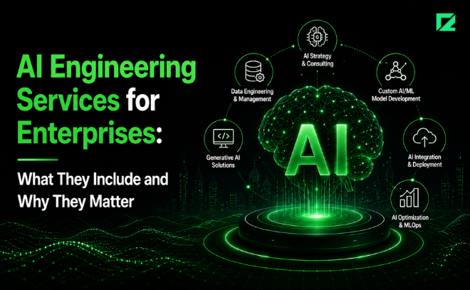
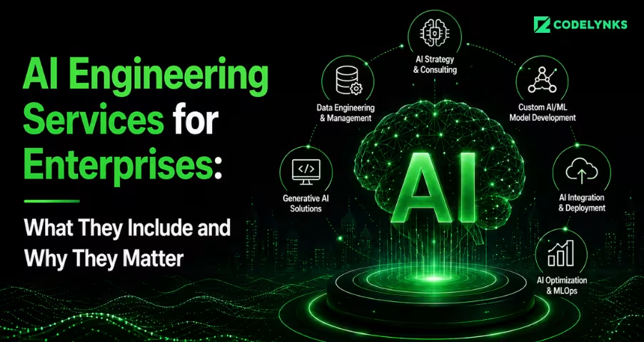
AI engineering services for Enterprises are becoming essential as organizations move from AI experimentation to production deployment. Most enterprises do not fail at AI because of bad ideas. They fail at the build. A model that works in a notebook is not a system that works in production. AI engineering services close that gap by turning AI concepts into scalable, secure, and reliable business systems.
This post explains what enterprise AI engineering services cover, why large organizations need them, and how to pick a provider that ships.
What are AI engineering services?
AI engineering services are professional services that design, build, deploy, and maintain AI systems for production use. They combine data engineering, machine learning, software engineering, and operations to deliver systems that run at scale. The work ends with a live system, not a slide deck.Strategy tells you where to go. AI engineering gets you there.
Why enterprises need AI engineering services
Enterprises carry weight that startups do not. Legacy systems, strict compliance, large data volumes, and many stakeholders all slow AI down. Building AI inside this environment takes engineering discipline, not just data science.
Three problems push enterprises toward outside engineering help:
The skills gap. Senior ML and AI engineers are scarce and expensive to hire.
The production gap. Internal teams build prototypes that never reach users.
The integration gap. New AI has to connect to systems built decades ago.
AI engineering services solve all three. They bring the people, the production discipline, and the integration experience in one team.
Core AI engineering services for enterprises:
A full provider covers the lifecycle from data to deployment. Here are the services that matter most.
Data engineering and pipelines: AI runs on clean, accessible data. Engineers build pipelines that collect, clean, and move data to where models need it. They fix quality problems that block accuracy. Without this layer, nothing downstream works.
Custom machine learning development: Off-the-shelf tools rarely fit a complex enterprise need. Engineers build and train custom models for your specific problem. This covers prediction, classification, recommendation, forecasting, and anomaly detection.
Generative AI and LLM integration: Many enterprises now want large language models inside their products and workflows. Engineers integrate LLMs for search, support, document processing, and content generation. They add retrieval, guardrails, and evaluation so the output stays accurate and safe. Popular foundation model providers include OpenAI and Anthropic, whose models are widely used in enterprise AI applications.
AI system architecture and integration: A model is one part of a system. Engineers design the full architecture and connect the AI to your existing stack, including CRMs, ERPs, and internal tools. They plan for scale, cost, and security from the start.
MLOps and deployment: Models need a path to production and a way to stay healthy there. MLOps services cover deployment, versioning, monitoring, and retraining. This is the discipline that keeps AI working after launch, when most projects quietly break.
Model evaluation and governance: Enterprises answer to regulators, auditors, and customers. Engineers build evaluation and governance into the system. They test for accuracy, bias, and safety, and they document how the system makes decisions.
Enterprise use cases for AI engineering: AI engineering services apply across functions and industries. Common examples:
Function
Example application
Customer service
LLM assistants that resolve tickets and route cases
Finance
Fraud detection and risk scoring at scale
Operations
Demand forecasting and supply chain optimization
Sales and marketing
Lead scoring and personalization engines
Legal and compliance
Document review and contract analysis
Manufacturing
Predictive maintenance on equipment
The pattern is the same in each case. A repeatable, data-heavy task becomes faster and more accurate with a system built around it.
Benefits of enterprise AI engineering services
Done well, these services produce results you can measure:
Faster delivery. A specialist team ships in months, not years.
Lower risk. Phased builds let you stop before large spending.
Production reliability. Systems built by engineers stay up and stay accurate.
Cost control. Right-sized architecture keeps inference and infrastructure costs in check.
Internal capability. Good providers transfer knowledge so your team can run the system.
The point is not AI for its own sake. The point is a working system tied to a business metric.
How to choose an AI engineering services provider
Not every vendor that says AI can build production systems. Screen for four things:
Production track record. Ask for live systems with real users, not pilots.
Full-lifecycle capability. They handle data, build, deployment, and support.
Enterprise experience. They know compliance, security, and legacy integration.
Phased engagements. You can exit between phases and keep what was built.
Walk away from anyone who quotes a fixed price before seeing your data. Serious engineers scope after they understand the problem.
What it costs and how long it takes
A proof of concept usually runs a few weeks and lands in the low tens of thousands. A full production engagement runs three to six months and into six figures for an enterprise.
Three factors move the numbers: data quality, compliance requirements, and integration depth. Messy data and deep legacy integration cost the most. Ask for a phased quote so you control spend at each stage.
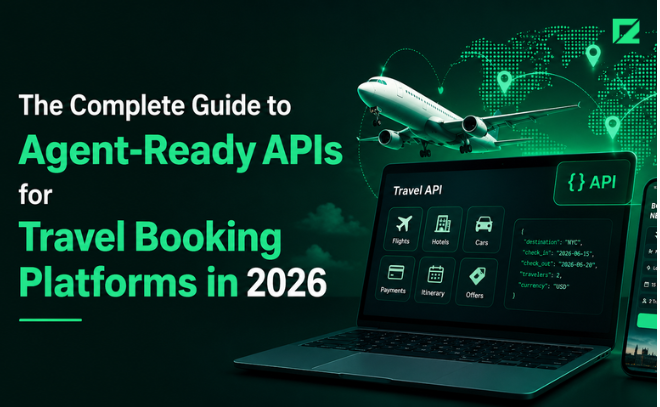
Agent-Ready Travel APIs are quickly becoming a critical requirement for online travel agencies (OTAs), airlines, hotels, and hospitality platforms. In March 2026, OpenAI pulled its travel booking capability from ChatGPT due to API reliability challenges
In March 2026, OpenAI pulled its travel booking capability from ChatGPT. The stated reason was complexity. The actual reason, documented across multiple platform post-mortems, was API reliability. Browser-automation agents navigating OTA websites were looping for 5 to 30 minutes before abandoning bookings on date pickers, fare selectors, and identity verification screens. The failure rate was too high to offer a credible product.
The Google I/O announcement in May 2026 made clear that agentic travel booking is not a future experiment. Google’s AI agents now query flight and hotel inventory through direct API integrations with Booking.com and major airline GDS systems. Skyscanner, Sabre, and others are building agent-compatible API layers. The industry is not asking whether agentic booking will happen. It is asking which platforms will still have transaction volume when it does.
If your booking platform serves outbound travelers and your API was designed for a human user sitting at a browser, you have a specific set of performance and reliability problems that will surface under agent load. This post names them.
Why Human-Optimized APIs Break Under Agent Traffic
Human users tolerate a 5-second search timeout and retry manually. AI agents abandon the session at 800 milliseconds and move to the next provider in their comparison set. This is not a theoretical preference. It is the observable behavior in production agentic systems, documented in PhocusWire’s analysis of major booking platform API performance under agent-led traffic.
The mismatch runs deeper than latency:
Session assumptions. Most OTA session management was designed around a human browsing pattern: search, browse, select, fill a form, pay. Sessions expire in 15 to 20 minutes because humans abandon carts. An AI agent operates in parallel across multiple booking options. It may hold a search result for 90 seconds while evaluating competing options. When it returns to complete the booking, the session is expired, the fare is stale, and the agent records a failure.
Error vocabulary. OTA APIs frequently return HTML error pages for backend failures, 302 redirects for authentication timeouts, and unstructured JSON payloads with human-readable error messages. A human reads “your session has expired, please search again” and acts on it. An agent parser sees a 200 response with an HTML body and records a booking confirmation. The confusion triggers support tickets, double-charges, and ghost reservations.
Rate limit design. Rate limits on most travel APIs were calibrated against human browsing patterns: low average request volume, occasional bursts during promotions. An agent comparing five flights across three platforms generates 15 to 20 API calls in 30 seconds. Most OTA rate limit configurations classify this as scraper behavior and block it.
The Agent-Ready API Scorecard (ARAS)
Codelynks uses the Agent-Ready API Scorecard to assess booking platform APIs before performance engineering work begins. ARAS evaluates five dimensions.
Dimension 1: Latency
Target P99 response times for agent-compatible booking APIs:
Availability/search: under 800 milliseconds
Fare verification (re-quote at booking initiation): under 1.5 seconds
Booking initiation (pre-confirmation step): under 2 seconds
Payment confirmation: under 3 seconds
A composite South Asian OTA we work with, handling 80,000 monthly leisure travel transactions for outbound Indian travelers, measured their P99 search latency at 4.2 seconds before optimization. That is within acceptable range for a human user with a loading spinner. For an agent comparing itineraries across five platforms simultaneously, it means the OTA’s results arrive after the agent has already made a preliminary selection elsewhere.
Dimension 2: Determinism
Agent-compatible APIs must be idempotent for booking requests. If an agent sends a booking request and receives no response (network timeout), it needs to retry without creating a duplicate booking. Idempotency keys at the booking endpoint prevent ghost reservations. Most OTA booking APIs do not support idempotency keys.
Fare determinism is equally critical: the fare returned in a search result must be honerable when the agent presents it at booking initiation. A fare change between search and booking (a common OTA behavior during high-demand periods) breaks the agent’s decision logic and results in an abandoned transaction.
Dimension 3: Session Resilience
Agent-compatible session design requires:
Session TTL of at least 10 minutes from the last API call, not from session creation
Token-based authentication that can be refreshed without full re-authentication
No CAPTCHA or secondary authentication challenges on machine-to-machine API paths
Consistent state between parallel API calls on the same session (a common failure in multi-datacenter OTA deployments)
The CAPTCHA problem is significant. Multiple agentic platforms have documented CAPTCHA walls appearing mid-session on OTA APIs, breaking the booking flow completely. CAPTCHA is legitimate fraud prevention for anonymous browser traffic. It is not appropriate on a credentialed API path.
Dimension 4: Error Grammar
A machine-readable API error response must include:
A numeric error code (not a human-readable string)
An error category (client error, server error, availability error, payment error)
A retry guidance field (should the agent retry immediately, after a delay, or not at all)
A trace ID for support escalation
OTA APIs that return HTTP 200 with an error message in the body, or HTTP 500 with an HTML maintenance page, are not machine-readable. An agent that cannot parse an error cannot respond to it intelligently.
Dimension 5: Concurrency
Agent traffic is bursty and parallel. A single agent managing a complex trip itinerary (outbound flight, hotel, transfers, inbound flight) may issue 40 to 60 API calls in under 2 minutes. Rate limit configurations must distinguish between:
Anonymous scraper traffic (high volume, randomized patterns, no session continuity)
Human browser traffic (lower volume, irregular timing, session-cookie authenticated)
Most OTA rate limit implementations treat all high-volume traffic as scraper traffic. This blocks credentialed agents and creates a competitive disadvantage for platforms that do not build agent-specific API tiers.
The Summer 2026 Stakes
Peak travel season begins in June. For outbound Indian travelers, the June to August window is the highest booking volume period. Agentic booking is no longer experimental for this demographic: Google’s AI travel tools are already integrated into search results, and Indian travelers are increasingly beginning trip planning through AI assistants rather than directly visiting OTA websites.
OTAs that do not surface correctly in agent-mediated comparison will lose bookings that never register as lost. There is no abandoned cart notification when an agent silently redirects to a competitor.
The Bain and Company analysis of airline readiness for agent-led bookings reached a blunt conclusion: most airlines and their distribution partners are not ready. The same finding applies to OTA booking APIs. Readiness is measurable, and the measurement starts with ARAS.
What This Means for Travel and Hospitality Leaders
The most concrete step available this week is an API call trace audit: record actual API call sequences from production traffic and identify the 10 requests with the highest P99 latency, the 5 most common error response types, and the session expiry rate during search-to-booking flows. That audit will tell you exactly which ARAS dimension to address first.
OTAs that treat this as a “build an AI chatbot” problem are solving for the wrong surface. AI agents do not need your chatbot. They need your booking API to return a fare, confirm idempotently, and fail with a machine-readable error when something goes wrong. That is a backend engineering problem, and it has a clear solution.
About the author: The Codelynks engineering team has delivered API performance engineering and platform reliability projects for travel, logistics, and financial services platforms across South Asia and the GCC. Connect on [LinkedIn](https://www.linkedin.com/company/codelynks).*
Smart meter infrastructure architecture is becoming the most critical success factor in India’s RDSS smart metering program. While millions of smart meters are being deployed nationwide, the real challenge lies in building scalable AMI platforms, MDMS systems, and data integration layers that transform meter readings into actionable grid intelligence.
A smart meter records a reading every 15 minutes. At 1 million installed meters, that is 2.9 billion data points per month. At RDSS’s full target of 250 million meters, that is 720 billion data points per month. Most DISCOM IT environments were built for monthly manual meter readings and a handful of operational reports. The gap between what is being installed and what can be operationally absorbed is not a hardware problem. It is an architecture problem.
This post covers what that architecture needs to look like, where DISCOMs and their technology partners typically underinvest, and a framework for building edge-capable AMI infrastructure that scales to RDSS targets.
The meter is the easy part: The three smart meter communication technologies deployed under RDSS are RF mesh, GPRS/cellular, and Wi-SUN (a wireless standard designed specifically for smart utilities). All three are mature. Comminent shipped 500,000 Wi-SUN modules in 2026 alone. Hardware procurement, while challenging at 250 million units, is a solvable supply chain problem.
A robust Smart Meter Infrastructure Architecture ensures that data collected from field devices can be processed, validated, and distributed across billing, outage management, and grid operations systems without creating bottlenecks.
What the meter itself does not solve:
How meter data travels from field to head-end system (HES), and at what latency
How the HES handles data validation, gap-filling, and transformation before feeding the Meter Data Management System (MDMS)
How the MDMS exposes consumption, tamper alerts, and demand-side signals to billing, outage management, and load forecasting systems
What happens when the communication network has 40% packet loss in a monsoon season (which is common in rural rollout areas)
The pv-magazine analysis from January 2026 framed this correctly: smart meters are being recognized as edge sensors, not just billing devices. That reframing has operational consequences. An edge sensor is part of a compute architecture. A billing device is just an input to an invoice.
The Smart Grid Edge Architecture Ladder (SGEAL): Codelynks uses the Smart Grid Edge Architecture Ladder to help DISCOMs and their system integrators assess where they currently operate and what the next investment should be. SGEAL has four levels.
Level 1: Collection: The foundation of any AMI deployment. The meter communicates to the Head-End System via the field communication network (FCM). At Level 1, the primary concerns are:
FCM reliability: What percentage of meters successfully communicate each push cycle? A 95% push rate sounds acceptable until you realize the 5% that fail are not random; they cluster in specific geography, device models, or network conditions.
HES capacity: The HES must ingest, validate, and timestamp incoming reads without queue buildup. An under-specified HES becomes a bottleneck at scale.
Data gap handling: Reads that fail to arrive must be flagged, interpolated (where policy allows), and marked for back-read retry. This logic must be in the platform from day one.
Level 2: Processing: At Level 2, validated reads flow from the HES to the MDMS. The MDMS is where meter data becomes structured consumption data. Key capabilities at this level:
Interval data validation rules: Spike detection, reverse energy flags, and meter health checks
Tamper detection: Current reversal, magnetic interference, neutral disturbance
Billing determinant calculation: Time-of-use (ToU) calculation requires interval-level data aligned to tariff periods
Revenue assurance: Estimated versus actual consumption tracking at the feeder and subdivision level
A state DISCOM technology partner in south India that we supported through an AMI rollout across 2.3 million consumers ran their MDMS on a platform originally designed for 200,000 meters. When the first 800,000 meters went live, the MDMS validation queue fell 18 hours behind real time. Billing runs were triggering on partially validated data. The fix required a horizontal scaling of the MDMS processing tier and a complete redesign of the job scheduling architecture. Neither was in the original scope.
Level 2 is where most RDSS implementations will encounter their first serious operational incident.
Level 3: Intelligence; At Level 3, the MDMS begins feeding operational systems with near-real-time signals. This is where smart metering crosses from billing infrastructure to grid operations tool.
Real-time load forecasting: 15-minute interval data at the feeder level enables intraday load curve prediction with accuracy that manual readings cannot approach
Demand response: Customers on time-of-use tariffs can receive signals to shift load off-peak. The meter must be capable of receiving and executing remote commands, not just transmitting reads.
Outage detection: A meter that stops reporting is likely experiencing an outage. When cross-referenced against feeder-level topology data, smart meter silence maps directly to fault location.
Non-technical loss (NTL) analytics: Comparing meter consumption against feeder-level injection identifies theft and billing anomalies at scale.
Level 3 requires a data integration layer between the MDMS and the DISCOM’s SCADA, GIS, and customer care systems. This integration is typically absent in year-one AMI deployments.
Level 4: Orchestration: At Level 4, the AMI infrastructure becomes a platform for distributed energy resource (DER) management. This level includes:
Integration with rooftop solar generation meters and net-metering APIs
EV charging load management via smart charging stations that respond to grid state signals
Demand-response automation: Rule-based or AI-driven load-shedding decisions executed at the meter level without manual intervention
V2G readiness: Vehicle-to-grid energy flows require bidirectional meter capability and real-time settlement infrastructure
Most DISCOMs in India are operating at Level 1 or early Level 2 as of mid-2026. Level 4 is a 2028 to 2030 target for the leading utilities. The Ladder is useful because it gives technology partners a clear vocabulary for where investment should go next, and what dependencies exist between levels.
Utilities that invest early in Smart Meter Infrastructure Architecture gain a significant advantage in operational scalability, revenue assurance, and grid modernization compared to utilities that focus only on meter procurement.
The Three Infrastructure Decisions That Determine RDSS Outcomes
Decision 1: Centralized versus distributed HES topology. A single centralized HES is simpler to manage but creates a single point of failure and a scaling ceiling. A distributed HES with regional concentrators adds operational complexity but handles the 250-million-meter target without a full-platform replacement. This decision is very difficult to reverse once meter communications are provisioned.
Decision 2: MDMS as a product versus MDMS as a platform. Most procurement decisions treat the MDMS as a commercial-off-the-shelf product purchase. At RDSS scale, the MDMS must behave as a platform: exposing APIs for downstream consumption, supporting custom validation rule sets by state or tariff structure, and scaling its processing tier independently of its storage tier. Platforms that cannot separate compute from storage will hit a scaling wall.
Decision 3: Integration first, analytics second.** The market for smart meter analytics dashboards is crowded. The market for reliable MDMS-to-operational-system integration is not. DISCOM leadership consistently requests analytics before ensuring the underlying data pipeline delivers complete, validated reads. Analytics built on incomplete data produce decisions worse than no analytics at all.
What This Means for Energy and Utilities Leaders
If your DISCOM or technology partner is currently planning or executing an RDSS AMI rollout, the single most valuable action this week is a Level 2 assessment: what is your MDMS processing capacity at 100%, 200%, and 500% of current installed meter count? If the answer is uncertain, the architecture is not ready for the rollout it will encounter.
RDSS funding ends the hardware procurement problem. It does not end the engineering problem. The 250 million meters being installed over the next three to four years will generate data. The question is whether that data flows into operational decisions or into a storage system nobody queries.
The platforms that solve the integration architecture before the meters arrive will spend their operational budget on grid optimization. The platforms that solve it after the meters arrive will spend it on data quality remediation.
About the author: The Codelynks engineering team has delivered IoT data pipeline and edge computing projects for utilities and infrastructure clients across India and the Middle East. Connect on LinkedIn
Conclusion
The future success of RDSS depends not only on meter deployment but also on building a resilient smart meter infrastructure architecture capable of supporting billions of readings, advanced analytics, and distributed energy resources.
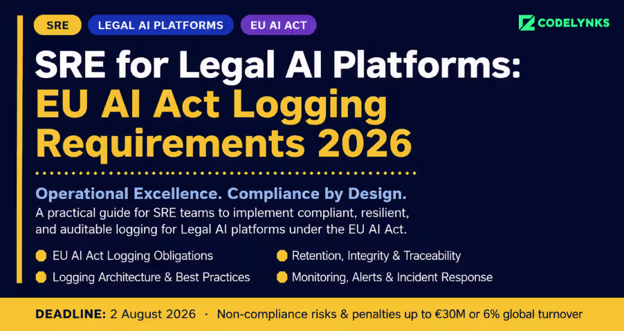
EU AI Act Logging Requirements are becoming a critical compliance concern for Legal AI platforms. An e-discovery platform that goes dark during a document production deadline does not just have a reliability problem—it has a liability problem.An e-discovery platform that goes dark during a document production deadline does not just have a reliability problem it has a liability problem. Legal software has always carried unusual reliability stakes: court filing deadlines are not negotiable, discovery windows are not extendable because a vendor’s API timed out, and privilege review workflows cannot be reconstructed from memory if audit trail logs are incomplete. The EU AI Act adds a new layer to this. From August 2, 2026,
AI systems used in the administration of justice and deployed in legal proceedings are classified as high-risk under Annex III. Article 12 requires automatic event logging sufficient to enable post-hoc reconstruction of the system’s behavior. Article 9 requires continuous risk management throughout the system’s lifecycle. For LegalTech platforms building on AI e-discovery classification, contract review automation, predictive case analytics, document privilege tagging the observability requirements are not engineering enhancements. They are compliance prerequisites.
What the EU AI Act Actually Requires from Legal AI Systems
The EU AI Act’s high-risk obligations under Annex III cover AI systems used by courts, public prosecutors, and legal aid entities as well as AI used in legal proceedings more broadly. The boundary is broader than many LegalTech vendors assume. AI-powered document review tools used in litigation, contract analysis systems used to support legal decisions, and predictive analytics tools used to assess litigation risk are all candidates for high-risk classification, depending on how they are deployed.
The two technical obligations that matter most to SRE and platform teams are Article 9 (risk management) and Article 12 (logging).
Article 9 requires a risk management system that runs throughout the AI system’s lifecycle not a one-time assessment. It requires continuous identification and mitigation of risks, with documented procedures for testing and monitoring. For a production AI system, this translates to: defined performance thresholds, automated monitoring that flags deviation, documented incident response procedures for AI-specific failure modes (model drift, hallucination, retrieval failure), and regular validation against a labeled test set.
Article 12 requires automatic event logs that capture the operating conditions of the system, the inputs processed, and the outputs generated. The logs must be generated automatically, stored in a format that is tamper-evident and retrievable on request, and retained for a period commensurate with the system’s use.
Logging that satisfies your engineering team’s debugging needs and logging that satisfies an EU AI Act audit are not the same thing. Build for the audit.
Why Legal AI Is High-Risk (and Why Your Vendor May Not Have Told You)
Many LegalTech vendors have been slow to classify their products under the EU AI Act because the classification requires an honest assessment of how the product is actually used not how the marketing materials describe it.
The critical question is whether the AI system’s output influences or informs a legal decision affecting an individual’s rights, legal status, or access to justice. A document review tool that classifies documents as privileged or non-privileged influences which documents a court will see. A contract analytics system that flags clauses as risky influences negotiation decisions with material legal consequences. A predictive litigation analytics tool that scores case strength influences settlement decisions that directly affect parties’ financial and legal positions.
Each of these use cases has a plausible argument for high-risk classification under Annex III. The vendor’s classification decision does not relieve the deploying organization of its compliance obligation. Under the EU AI Act, both providers (vendors building AI systems) and deployers (law firms and legal departments using them) carry obligations. If the vendor has not conducted a conformity assessment, the deployer must assess whether the system they are using meets the Article 9 and 12 requirements and document that assessment.
The question is not whether your legal AI system will face a regulatory review. It is whether you will be able to reconstruct what it did when that review happens.
The Legal AI Observability Stack (LAOS)
The LAOS defines four layers of observability that a legal AI platform must instrument to meet EU AI Act requirements and maintain operational reliability.
Layer 1: Infrastructure and service health
Standard SRE observability: service uptime, latency percentiles (p50, p95, p99), error rates, and infrastructure saturation. This layer is necessary but not sufficient for EU AI Act compliance. Most platforms already have it. Acceptance criterion: dashboards showing current service health are available to on-call engineers within 60 seconds; alerts fire within two minutes of a threshold breach.
Layer 2: AI pipeline observability
Monitoring specific to the AI components: model inference latency, retrieval latency (for RAG-based systems), embedding generation time, and input/output token counts. This layer enables performance debugging of AI-specific failure modes that infrastructure monitoring does not capture. Acceptance criterion: per-request AI pipeline latency is measurable and alertable independently of application-level latency.
Layer 3: Audit-grade inference logging
This is the Article 12 layer. Every inference call must generate a structured log record containing: document or query identifier (not the raw document content a hash or ID linking to a retrievable reference), model version ID, retrieval context used (for RAG systems which documents were retrieved and their identifiers), model output (classification label, confidence score, or generated text), timestamp (UTC, millisecond precision), and session or workflow identifier. Logs must be append-only, stored separately from the operational database, and retrievable by inference ID. Acceptance criterion: you can retrieve the complete inference record for any individual document review decision within one hour of a request.
Layer 4: Compliance monitoring and drift detection
Automated monitoring of the AI system’s behavior over time: output distribution drift (are classification decisions shifting toward one label?), inter-rater agreement monitoring (for systems where human review follows AI classification is the override rate changing?), and model version tracking. The compliance monitoring layer generates the evidence for Article 9’s continuous risk management requirement. Acceptance criterion: a compliance dashboard shows output distribution, override rate, and model performance metrics on a rolling 30-day basis; anomalies generate an incident ticket automatically.
Incident Response When the Stakes Are Discovery Deadlines
Legal software incidents are different from consumer application incidents in one significant way: the business impact of downtime is often tied to a specific external deadline that cannot be moved. A court-ordered document production is due on a specific date. A contract signing deadline is non-negotiable. A regulatory filing window does not extend because a vendor’s infrastructure had an outage.
This changes the calculus on recovery time objectives (RTO). In a standard application, an RTO of four hours is acceptable for non-critical services. In a legal platform, an RTO of four hours during an active discovery window is a professional liability event.
The legal AI platform incident response playbook must include:
Pre-incident: Documented understanding of active matters with imminent deadlines. The on-call engineer should have visibility into whether any matters have a filing or production deadline within the next 48 to 72 hours. This is business-context awareness that most SRE teams do not have.
During incident: A communication protocol for notifying affected customers within fifteen minutes of a P1 incident declaration before resolution. Legal teams need time to activate backup processes (manual review, alternative tools). Fifteen minutes is tight. It requires automation, not a manual Slack message.
Post-incident: A structured incident report that includes which AI inference operations were affected, whether any outputs generated during the incident window should be considered unreliable, and whether affected customers need to re-run any document reviews. This is the intersection of incident management and EU AI Act Article 12 the incident report is part of the audit trail.
An LPO firm we work with that handles cross-border contract litigation for UK clients had a production incident during a document production sprint. The AI classification service was intermittently returning incorrect labels for 90 minutes. They caught it through anomaly monitoring on their output distribution (an unusual spike in “non-responsive” classifications on documents that their experienced reviewers would have flagged differently). Because they had Layer 3 logging in place, they could identify exactly which documents had been classified during the incident window and queue them for human re-review. Without the inference-level log, they would not have known which documents to re-check.
Building the Audit Trail Without Killing Performance
The most common objection to inference-level logging is performance impact. Logging every inference call with a structured record adds latency to the inference path. At high volume, it can also add significant storage cost.
Three architecture patterns manage this without compromising logging completeness:
Async logging with buffered writes: Write inference logs to an in-memory buffer and flush asynchronously to the log store. The buffer flush interval should be short enough that logs are persisted within seconds. The risk log loss during a process crash is acceptable if you have structured retry logic on the write side and a dead-letter queue for failed writes.
Log separation from application database: Store inference logs in an append-only log store (AWS CloudWatch Logs, Google Cloud Logging, or a dedicated time-series log store) separate from the application database. This prevents inference log volume from affecting application database performance and simplifies the tamper-evidence requirement.
Content hashing, not content storage: Log the hash of the input document content, not the document text itself. The hash provides a cryptographically verifiable reference to the exact input without storing privileged legal documents in your log store. The original document remains in the matter management system; the log proves which document was processed at what time.
What This Means for Legal Technology Leaders
The EU AI Act’s August 2, 2026 deadline is the floor, not the ceiling. The enforcement wave that follows will create a body of case law and regulatory guidance that raises the bar for what “compliant” means. Legal AI platforms that build to minimum compliance now will need to iterate as guidance clarifies.
The steps you can take this week without engaging anyone externally: review your current inference logging against the Article 12 checklist. Can you reconstruct the complete decision record for any individual document classification within one hour? If the answer is no, that is your compliance gap and it is the one that carries direct regulatory exposure.
Then assess your RTO for your AI classification service. If it is measured in hours, not minutes, build the pre-incident deadline visibility and the fifteen-minute customer notification automation before the next deployment cycle.
About the author: The Codelynks SRE team has built observability and reliability stacks for legal document intelligence and compliance platforms across Southeast Asia and the UK. Connect on LinkedIn
FAQ
Are legal AI systems classified as high-risk under the EU AI Act?
AI systems used in the administration of justice, legal proceedings, and legal decision support are classified as high-risk under Annex III of the EU AI Act. This includes e-discovery platforms, contract analysis systems, and predictive litigation analytics tools that influence legal decisions affecting individual rights.
What does Article 12 of the EU AI Act require for logging?
Article 12 requires automatic, tamper-evident event logging that captures the operating conditions, inputs, and outputs of each AI system interaction. Logs must be retrievable on regulatory request and retained for an appropriate period. Aggregate or batch logs do not satisfy the requirement.
Who is responsible for EU AI Act compliance the LegalTech vendor or the law firm?
Both. Providers (vendors building AI systems) must conduct conformity assessments and maintain technical documentation. Deployers (law firms and legal departments using the systems) must ensure the systems they use meet Article 9 and 12 requirements. Both parties carry obligations.
How does Article 12 logging differ from standard application logging?
Standard application logs capture errors, performance events, and system state for debugging. Article 12 logs must capture the specific inputs processed and outputs generated by the AI system at the individual inference level, with enough detail to reconstruct any specific decision post-hoc. The purpose is regulatory audit, not debugging.
5. What is a realistic RTO for a legal AI platform during an active discovery window?
During an active discovery window with an imminent production deadline, an RTO measured in hours creates professional liability exposure. Legal AI platforms should target a 15 to 30 minute RTO for their AI classification services during active matters, with pre-incident deadline visibility to inform incident triage prioritization.
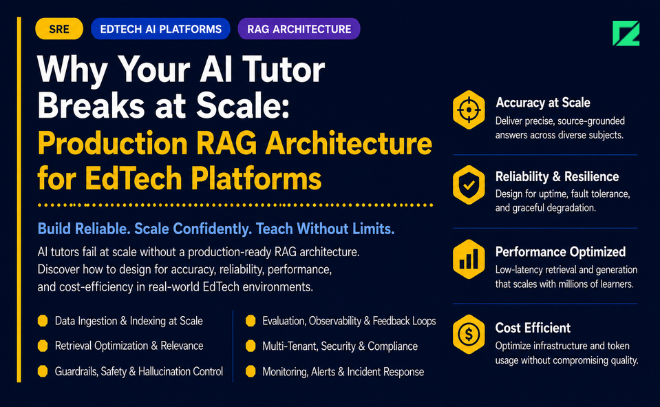
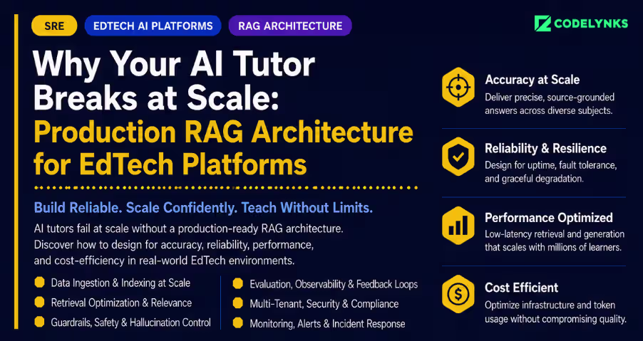
A mid-size ed-tech platform in India launched their AI tutor in January 2026. In the demo, it answered curriculum questions in 1.2 seconds with 94% accuracy against their grading rubric. In the classroom pilot with 800 students three months later, it averaged 8.7 seconds per response, hallucinated chapter numbers that did not exist in the NCERT textbooks, and failed entirely when a student asked a question that bridged two subject domains. The architecture that worked in the demo was vector RAG over a flat document store. The architecture that would have survived the classroom was not.
This gap is not unique to that platform. Most EdTech teams building AI tutors in 2026 are deploying architectures that are optimized for demo accuracy and underspecified for production reliability. The research now backs what production deployments have been showing: RAG-based tutoring systems require a different architecture than general-purpose RAG, and the differences are not cosmetic.
Why Vector RAG Fails Curriculum Content at Scale
Vector RAG works by converting a query into an embedding and retrieving the nearest chunks from a document store. For general knowledge retrieval, this is adequate. For curriculum content, it has a structural mismatch.
Curriculum knowledge is relational, not spatial. A student asking, “Why does current increase when resistance decreases?” needs an answer that assumes they have already understood Ohm’s Law. If they have not, the correct answer is to explain the prerequisite first. Vector similarity cannot represent that dependency. The nearest chunks to the query are the most conceptually similar, not the most pedagogically appropriate.
The failure modes this produces in production: responses that assume prior knowledge the student has not acquired, answers that correctly reference a concept but in the wrong order for the student’s current level, and complete retrieval failures when a query involves concepts from two subject areas that were indexed separately.
The PRAG-EDU framework published in *Computer Applications in Engineering Education* this year showed that grade-aware RAG where retrieval is calibrated to a student’s historical module performance, produced a 23.7% improvement in BERTScore F1 over standard vector retrieval. The improvement came from adjusting which chunks were retrieved based on the student’s demonstrated competence level, not from changing the underlying model.
A vector similarity score is not a pedagogical prerequisite. GraphRAG understands that one concept must come before another. Vector RAG does not.
GraphRAG vs Vector RAG: The EdTech Architecture Decision
GraphRAG represents curriculum content as a knowledge graph; nodes are concepts, edges are prerequisite and co-requisite relationships, and each node carries metadata about Bloom’s Taxonomy level and grade alignment.
When a student asks a question, GraphRAG retrieves not just the most similar chunk but the contextually adjacent concepts in the learning graph. This enables the tutoring system to answer the question, identify what the student needs to understand next, and detect gaps in foundational knowledge three things a vector store cannot do.
The practical objection is build cost. GraphRAG requires upfront curriculum ontology work someone must map the prerequisite relationships in your content. For a platform with 10,000 hours of NCERT-aligned content across 12 subjects, that is a significant indexing project.
The answer is to start with GraphRAG for high-stakes subject areas (mathematics, physics) where prerequisite dependencies are strict and the cost of wrong retrieval is highest, and use hybrid retrieval (graph + vector) for subjects where the knowledge structure is more associative (history, literature). The LPITutor system (published in PMC 2026) demonstrated this hybrid approach at the curriculum scale, using RAG with structured prompt engineering to handle both factual and explanatory query types.
LLM-agnostic architecture is worth addressing separately. The model behind your tutor will change probably annually. Every system prompt, retrieval pipeline, and session memory structure should be model-independent. Platforms that hardcoded GPT-4 or Gemini 1.5 Pro into their retrieval logic are rebuilding integration layers each time a better model ships.
The Five Production Failure Modes in AI Tutoring Systems
Based on deployments we have run and audited, the five failure modes that cause AI tutors to break in classroom conditions are consistent:
Failure Mode 1: No session memory isolation. Multiple students use the same system. Without session-level memory isolation, retrieval contexts bleed between sessions. A question from one student’s earlier session influences the next student’s answer.
Failure Mode 2: Flat document chunking. Textbook chapters chunked at fixed token intervals break concept boundaries. A 512-token chunk that starts mid-explanation and ends before the example is unretrievable for any meaningful query. Chunking must respect semantic boundaries paragraphs, concept blocks, and worked examples.
Failure Mode 3: No query classification. “What is the formula for kinetic energy” and “I don’t understand momentum” require different retrieval strategies. Without a query classification layer that routes to factual retrieval vs explanatory retrieval vs diagnostic retrieval, every query hits the same pipeline with the same retrieval parameters.
Failure Mode 4: No latency budget enforcement. A tutoring system in a live classroom has a usability ceiling around 3 to 4 seconds. Beyond that, students disengage. Most teams discover this threshold in production. Retrieval latency must be measured per pipeline stage and bounded, not monitored passively.
Failure Mode 5: Hallucination in low-retrieval-confidence scenarios. When the retrieval stage returns low-confidence results (the question is outside the indexed curriculum), the model defaults to generating from training data. For NCERT-specific content, training data is often imprecise. The system needs an explicit fallback: “This question is outside the material for this course. Please ask your teacher.”
The Tutoring System Reliability Stack (TSRS)
The TSRS is a five-layer framework for evaluating and designing production AI tutoring systems. Each layer has a pass/fail criterion.
Layer 1: Knowledge Representation
Is your curriculum represented as a knowledge graph with prerequisite relationships or as a flat vector store? Pass: GraphRAG or hybrid graph/vector. Fail: flat vector store only.
Layer 2: Session Context Management
Does each student session have isolated memory, and is session context bounded by a token budget to prevent context window overflow over a 45-minute class period? Pass: isolated sessions with explicit context pruning. Fail: shared context or unbounded session memory.
Layer 3: Query Routing
Does the system classify queries into factual, explanatory, and diagnostic types before routing to retrieval? Pass: classification layer with distinct retrieval strategies per type. Fail: uniform retrieval pipeline for all query types.
Layer 4: Latency Governance
Is there a latency SLO per pipeline stage? Is the retrieval stage bounded independently from the generation stage? Pass: per-stage SLOs with circuit breakers. Fail: end-to-end latency monitoring only.
Layer 5: Confidence Gating
Does the system measure retrieval confidence and fall back to an out-of-scope response when confidence is below threshold? Pass: explicit confidence gate with tested fallback. Fail: model generates from training data when retrieval fails.
A platform that passes all five layers can be trusted in a live classroom. A platform that passes three is ready for supervised pilots. Fewer than three means the system needs architecture work before student-facing deployment.
What Latency Actually Costs in a Classroom
The counterintuitive number: a tutoring system averaging 6 seconds per response at 800 concurrent students consumes more tokens in retries and regeneration than in successful first-attempt completions. Students who do not get a response within 4 seconds re-submit the query. The system processes both. Reducing latency from 6 seconds to 3 seconds on a platform of this size reduced inference spend by 34% in one engagement, not by optimizing the model, but by fixing the retrieval architecture so regeneration requests dropped.
Your AI tutor’s latency problem is not a model problem. It is an architecture problem that your model is paying for.
The fix was hybrid retrieval (GraphRAG for structured concept queries, vector for open-ended questions), smaller semantic chunks with richer metadata, and a query classifier that routed 60% of queries to a cached factual response layer that did not invoke the LLM at all.
What This Means for EdTech Leaders
If you are in production with an AI tutor and have not audited against the five TSRS layers, do it this week. The audit is a one-hour structured review of your retrieval architecture, session management design, and latency data. It will surface the failure mode your platform is most likely to hit during scale.
Three actions you can take without engaging anyone:
1. Pull your median response latency for the last 30 days and check whether it exceeds 4 seconds for any query category.
2. Ask your engineering team whether your retrieval pipeline uses the same strategy for factual queries and explanatory queries. If the answer is yes, you do not have query routing.
3. Run a test: ask your AI tutor a question that requires knowledge from two separate subject chapters. If the response retrieves only one chapter’s context, your knowledge representation is flat.
The EdTech platforms that will hold adoption in 2026 are the ones that close the gap between demo accuracy and classroom reliability. The architecture is understood. The build is an execution problem.
About the author: The Codelynks AI engineering team builds and audits LLM-powered applications for regulated and consumer-facing products across India and Southeast Asia.
FAQ’s
What is the difference between vector RAG and GraphRAG for AI tutoring systems?
Vector RAG retrieves content based on semantic similarity between a query and stored text chunks. GraphRAG represents content as a knowledge graph with explicit prerequisite and co-requisite relationships between concepts. For tutoring systems, GraphRAG is better suited because it can represent which concepts must be understood before others a relationship vector similarity cannot capture.
How fast should an AI tutor respond to be usable in a live classroom?
Based on classroom deployments, usability drops significantly beyond 4 seconds per response. Students re-submit queries after 4 to 5 seconds, which creates duplicate inference load and increases cost. A target of 2 to 3 seconds for most query types is achievable with a properly structured retrieval pipeline.
What is the Tutoring System Reliability Stack (TSRS)?
The TSRS is a five-layer evaluation framework for production AI tutoring systems developed by Codelynks. The five layers are knowledge representation, session context management, query routing, latency governance, and confidence gating. A system must pass all five layers before student-facing deployment at scale.
Can an AI tutoring platform work offline for students with poor connectivity?
Offline tutoring requires a fundamentally different architecture smaller, quantized models, on-device inference, and locally cached knowledge graphs. Recent research has demonstrated feasibility for constrained environments, but the current-generation RAG architectures described in this post require network connectivity to the retrieval and generation services.
How much does it cost to build a GraphRAG knowledge base for a K-12 curriculum?
The primary cost is ontology work mapping prerequisite relationships in the curriculum. For a 12-subject NCERT-aligned curriculum, this typically requires 6 to 10 weeks of curriculum specialist and engineering time. The technical infrastructure cost is lower than ongoing vector store embedding costs at comparable query volumes.
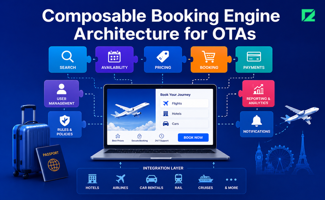
Composable booking engine architecture is reshaping how modern OTAs support AI booking agents, dynamic packaging, and API-first travel commerce.
Your booking engine was built for browsers. AI agents do not use browsers. Your Booking Engine Was Built for Browsers. AI Agents Do Not Use Browsers. The next wave of travel bookings will not come through a human typing into a search box. It will come through AI agents operating autonomously on behalf of travelers, calling your APIs directly to check availability, price, and confirmation. If your booking engine requires a browser session to complete a transaction, AI agents will route around you to a platform that does not.
A mid-size OTA operating across Southeast Asia came to us in mid-2025 with a problem that had become familiar: their booking engine, built on a monolithic PHP stack in 2018, was taking four months to ship a pricing rules change. Every new distribution channel, a new airline GDS connection, a new hotel chain API, required touching the same codebase and passing the same regression suite. Engineering velocity had collapsed. Revenue from new channels was being left on the table because the cost of integration had become prohibitive.
They shipped a composable booking architecture in seven months. Deployment cycles for individual services are now measured in days. Three new distribution channels went live in the first quarter after migration. This post explains the sequence we followed and where the decisions actually matter.
Why Monolithic Booking Engines Are Failing Now, Not Later
Monolithic travel platforms were designed for a single delivery channel: a web browser, with a human in the loop. That assumption is now incorrect on two fronts.
First, AI-powered booking agents, whether built on Claude, GPT-4o, or custom models, require structured API access to inventory, pricing, and availability. They do not render HTML. They do not fill in forms. They call REST or GraphQL endpoints and expect machine-readable responses. A monolithic booking engine that serves a rendered UI cannot serve an AI agent without significant reverse engineering.
Second, dynamic packaging has become the standard expectation for premium travelers. A flight, a hotel, an activity, and travel insurance, assembled into one iterable itinerary, confirmed in a single checkout. Monolithic platforms handle this through tightly coupled modules. When any one module changes, the whole checkout breaks. That coupling is why pricing updates take months.
> A monolithic booking engine is not a technical problem. It is a revenue ceiling.
The average composable-architecture OTA in 2026 deploys features 80% faster than a monolith-based competitor. That number tracks with what we observed with our Southeast Asian client.
The MACH Foundation in Travel Commerce
MACH stands for Microservices, API-first, Cloud-native, and Headless. In a travel context, this means:
Microservices: Each commerce function, flight search, hotel availability, rate calculation, checkout, confirmation, and post-booking management runs as an independent service with its own database, its own deployment pipeline, and its own failure boundary. A problem in the hotel availability service does not cascade to check-out.
API-first: Every function is exposed through a documented, versioned API before any frontend consumes it. This is the piece most travel platforms get wrong. They build the API as an afterthought to the UI. In a MACH stack, the API is the product. The UI is one consumer.
Cloud-native: Services scale independently. Flight search at peak demand requires different compute than post-booking email workflows. Pay-as-you-go scaling reduces infrastructure costs by 30 to 40% for seasonal travel businesses that see 5x demand swings.
Headless: The frontend presentation, whether a web app, a mobile app, a WhatsApp booking bot, or an AI agent, is decoupled from the backend commerce engine. Any channel can consume the same API. New channels add zero backend work.
> AI booking agents do not fill in forms. They call APIs. If your booking flow requires a browser session, an AI agent cannot book through you.
The Travel Stack Decomposition Sequence (TSDS)
We have run enough of these migrations to know that the sequencing matters more than the technology choices. This is the six-step decomposition sequence that has worked consistently.
Step 1: Inventory and Availability API: Extract the flight search, hotel availability, and activity inventory functions first. These are read-heavy, stateless, and cacheable. They cause the least disruption when extracted and they deliver the first visible performance win: faster search response times. Target: extracted within weeks 1 to 6.
Step 2: Pricing and Rate Engine: The rate calculation engine is the most complex extract because it carries the most business logic. Map every pricing rule before touching any code. Build contract tests against current behavior. Extract it to a dedicated service with its own test suite. Target: weeks 6 to 14.
Step 3: Checkout and Payment Orchestration: Checkout is the highest-stakes service because any failure here is a lost booking. Extract this after Steps 1 and 2 are stable. Build idempotency into every payment API call from the start. Integrate Stripe, Razorpay, or your regional gateway through an adapter layer so the payment provider can be swapped without touching checkout logic. Target: weeks 12 to 20.
Step 4: Dynamic Packaging Engine: Once inventory, pricing, and checkout are independent, dynamic packaging becomes straightforward: a composition service that calls the three downstream services, assembles an itinerary, and returns a single bookable product. This is the service that AI agents will call most frequently. Target: weeks 18 to 24.
Step 5: CMS and Content API: Destination content, hotel descriptions, activity details, and promotional banners are extracted to a headless CMS (Contentful, Sanity, or Storyblok are the common choices in travel). This eliminates the dependency between marketing content updates and engineering releases. Target: weeks 20 to 26.
Step 6: Frontend Delivery Layer: The last step is rebuilding the consumer-facing frontend against the new API layer. This is where most teams want to start. It is the wrong place to start. Build the API surface first. The frontend will be faster and cheaper to build when it does not have to work around backend constraints.
The OTA we worked with reached Step 4 before migrating their primary frontend. Three months before the frontend migration completed, they had already launched a WhatsApp booking channel and an API integration with a corporate travel management platform, both consuming the same new API layer.
Where Teams Underestimate the Work
Two areas consistently surprise teams mid-migration.
GDS integration complexity: Global Distribution Systems (Amadeus, Sabre, Travelport) expose SOAP-based APIs with response schemas that were designed before REST existed. Wrapping these in clean REST or GraphQL adapters is essential but time-consuming. Budget 4 to 6 weeks specifically for GDS adapter work. Do not absorb it into the inventory service timeline.
Booking state management: A booking in progress carries state across multiple services: seats held in inventory, a price locked in the rate engine, payment in process. In a monolith, a database transaction handles this. In a distributed system, you need explicit saga orchestration. The Saga pattern with choreography (services reacting to events) handles most travel booking flows. The Orchestrator pattern (a central service coordinating the saga) is better for complex multi-leg itineraries where rollback logic is intricate.
> The cost of a composable migration is front-loaded. The cost of staying monolithic is back-loaded and compounding.
What This Means for Travel Leaders
If you are running an OTA or a hotel booking platform with a monolithic core, three decisions this week will tell you whether you are on the right path:
Check whether your booking engine exposes any documented APIs today. If the answer is no, AI agent distribution is not accessible to you. That gap will widen through 2026 and 2027.
Ask your engineering team how long it takes to ship a pricing rule change end to end. If the answer is longer than two weeks, you are paying a compound productivity tax that TSDS Step 2 eliminates.
About the author: The Codelynks engineering team has designed and shipped commerce platforms and booking engines for travel, retail, and marketplace clients across Southeast Asia and the GCC. [Connect on LinkedIn](https://linkedin.com/company/codelynks).*
FAQ’s
What is composable booking engine architecture?
A composable booking engine separates each commerce function, flight search, pricing, checkout, and packaging into independent microservices that communicate via APIs. This allows each component to be updated, replaced, or scaled independently without affecting the others.
How long does a composable migration take for a mid-size OTA?
Following the Travel Stack Decomposition Sequence, a mid-size OTA with a team of six to eight engineers can complete a full composable migration in 24 to 30 weeks, with early wins from the inventory and pricing extractions visible within the first three months.
Can a composable booking engine serve AI booking agents?
Yes. This is the primary technical advantage of an API-first architecture. AI booking agents, operating autonomously on behalf of travelers, require REST or GraphQL endpoints. A monolithic booking engine that relies on browser sessions cannot serve these agents.
What is the difference between headless commerce and composable commerce in travel?
Headless separates the frontend from the backend via APIs. Composable goes further: every backend function is also an independent, swappable service. A headless OTA still has a monolithic backend. A composable OTA has both a decoupled frontend and a decoupled backend.
Which GDS systems are compatible with composable travel architectures?
Amadeus, Sabre, and Travelport all offer REST-based API access alongside their legacy SOAP interfaces. Building a clean adapter layer around GDS connections is standard practice in a composable migration and prevents GDS-specific quirks from leaking into the rest of the booking stack.
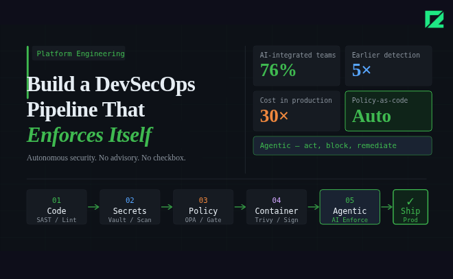
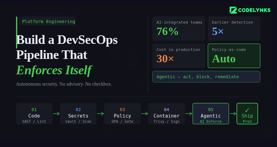
A security scan that runs after your build is not a DevSecOps pipeline. It is a security checkbox that runs after your build. The distinction matters because one approach catches vulnerabilities before they reach production, and the other hopes someone reads the report.
According to industry data from N-iX and DZone’s 2026 DevOps surveys, 76% of DevOps teams have already integrated AI into their CI/CD pipelines. The shift happening now is not just more tooling in the pipeline. It is tooling that can act, enforce, and remediate, not just report. This guide explains how to build a pipeline where security is a hard constraint, not an advisory. A modern DevSecOps pipeline integrates automated security checks into every CI/CD stage.
The Architecture of a Secure Pipeline
A DevSecOps pipeline has security controls at four stages: before the commit, during the build, before deployment, and in production. Each stage catches different classes of vulnerability. Skipping any stage creates a gap that will eventually be exploited.
Stage 1: Pre-Commit Hooks
Pre-commit hooks are the first line of defense. They run on the developer’s machine before code reaches the repository.
What to run at pre-commit:
Secrets scanning: Detect API keys, credentials, and tokens before they are committed. Tools: detect-secrets (Yelp), gitleaks, or truffleHog. Configure with a deny-list that matches your organisation’s credential patterns.
Linting and formatting: Enforce code style standards. Not strictly security, but a consistent codebase is easier to audit.
Infrastructure-as-code validation: If developers write Terraform or Kubernetes manifests, run a lightweight policy check (tflint, kubeval) to catch obvious misconfigurations before the commit reaches the pipeline.
Use the pre-commit framework (pre-commit.com) to manage hooks declaratively in a .pre-commit-config.yaml file, committed to the repository. This ensures every developer runs the same set of checks.
Stage 2: Build-Time Checks (Pull Request Gate)
Every pull request should trigger a suite of automated security checks that must pass before the branch can be merged. These are the pipeline gates.
Static Application Security Testing (SAST): Analyse source code for known vulnerability patterns without running the code. Tools: Semgrep (best open-source option), Checkmarx (enterprise), SonarQube with security rules. Configure severity thresholds: CRITICAL and HIGH findings block the merge, MEDIUM and LOW generate tickets.
Software Composition Analysis (SCA): Check every open-source dependency against known CVE databases. Tools: Snyk, OWASP Dependency-Check, GitHub Dependabot. Flag dependencies with CVE scores above your threshold. The biggest advantage of a DevSecOps pipeline is continuous security enforcement during development and deployment.
Infrastructure policy validation: Run Checkov or Terrascan against all Terraform and CloudFormation changes in the PR. Policy violations block the merge.
SBOM generation: Generate a Software Bill of Materials for the build artifact. Tools: Syft, CycloneDX. Store it as a build artifact. This is becoming a procurement requirement for enterprise and government customers.
Stage 3: Pre-Deployment Checks
Before any artifact reaches staging or production, validate the complete deployable unit, not just the source code.
Container image scanning: Scan the built container image, not just the application code. Base images carry their own vulnerabilities. Tools: Trivy (open source, fast), AWS ECR scanning, Google Artifact Analysis. Block deployment of images with HIGH or CRITICAL CVEs in base image packages.
Image signing and verification: Sign built images with cosign (Sigstore) and enforce signature verification at deployment time using a Kubernetes admission controller. This prevents tampering between build and deployment.
Kubernetes manifest validation: Validate deployment manifests against your security policies using Kyverno or OPA/Gatekeeper as an admission controller. Block pods running as root, containers without resource limits, and images from unauthorised registries.
Stage 4: Runtime Security Monitoring
Deployment is not the end of the security pipeline. Production has a different threat surface than the build environment.
Runtime threat detection: Tools like Falco (open source) or Sysdig detect anomalous behaviour in running containers: unexpected outbound connections, process executions that are not in the image, file system writes to unexpected locations. Alert on these immediately.
Periodic image rescanning: A CVE-free image today may be vulnerable tomorrow. Schedule weekly rescans of all images in your container registry. Automatically open tickets for newly discovered vulnerabilities in deployed images.
API anomaly detection: Unusual API call patterns, authentication failures above baseline, and privilege escalation attempts in production need automated detection and response. Define your baseline, set alerting thresholds, and create automated response playbooks for the highest-severity patterns.
Where Agentic AI Fits In
The 2026 evolution in DevSecOps is not just more tools. It is tools that can reason about context, suggest remediations, and act autonomously on low-risk findings.AI-powered monitoring is becoming a core capability in every enterprise DevSecOps pipeline.
AI-powered SAST tools can understand the data flow context of a vulnerability, not just its pattern signature. A SQL injection vulnerability in a function that only receives internally-validated input has a different risk profile than one receiving raw user input. Contextual analysis produces fewer false positives and more accurate severity ratings.
AI remediation suggestion at the pull request stage has demonstrated significantly higher fix rates than traditional vulnerability reporting. When a developer sees a suggested code change alongside the vulnerability finding, they fix it immediately. When they receive a ticket in Jira, it joins the queue.
Getting Started: The Minimum Viable DevSecOps Pipeline
If you are starting from zero, do not try to implement all four stages simultaneously. Build in this order:
Add secrets scanning as a pre-commit hook and as a pipeline check. This is the highest-severity gap in most pipelines and takes less than a day to implement.
Add SCA for dependency vulnerability scanning on every PR. Use Snyk or Dependabot. Configure automated PRs for patch-level updates.
Add SAST with Semgrep. Start with the community rulesets, tune the false positive rate for your codebase over the first month.
Add container image scanning with Trivy. Block deployment on CRITICAL CVEs, alert on HIGH.
Add infrastructure policy checks with Checkov. Define your top-10 must-enforce policies first.
Add runtime monitoring with Falco. Define alert rules for your most sensitive workloads first.
Steps 1-4 can be implemented within two weeks. Steps 5-6 require more planning but are achievable within a quarter.
Need Help With This?
Codelynks builds DevSecOps pipelines for engineering teams in regulated industries. If you need a security posture assessment or want to design a CI/CD pipeline with autonomous security enforcement, talk to our team at contact us
Cloud vendors raised prices in 2026. Egress fees for moving data from cloud to on-premise remain high. AI inference at scale is creating new latency constraints that central data centres struggle to meet. And data sovereignty regulations in the EU, India, and Southeast Asia are adding geographic constraints to workload placement.
All of these pressures point in the same direction: for specific workloads, moving compute closer to the data source, at the edge, is now the better architectural choice.
This post is a practical guide to when edge processing delivers a measurable advantage, what the architecture looks like in production, and where implementations typically go wrong.
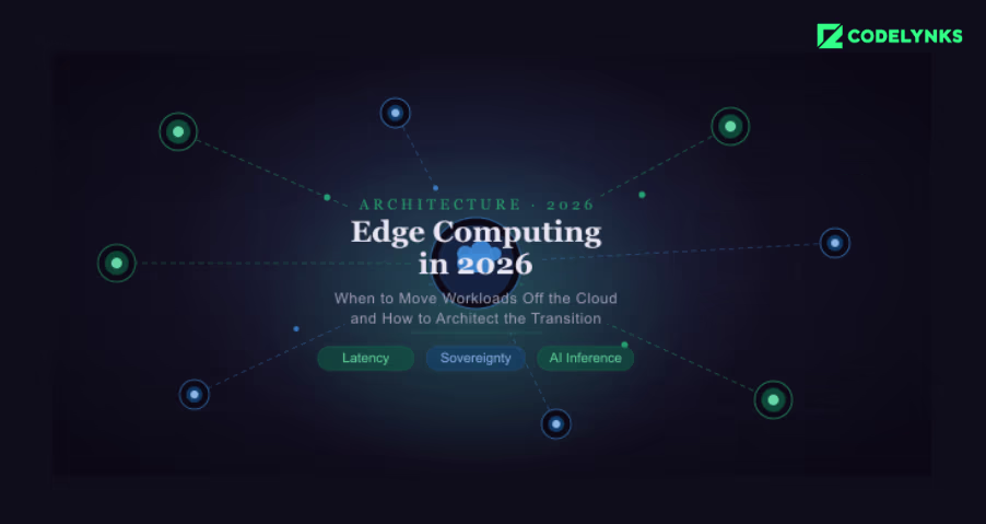
What Edge Computing Architecture Means in 2026
Edge computing is not a single architecture. The term covers three distinct deployment patterns, each solving a different problem.
CDN edge nodes: compute running at points of presence (PoPs) globally, typically 15-30ms from end users. Cloudflare Workers, AWS Lambda@Edge, and Fastly Compute fall into this category. Best suited for low-latency API responses, A/B testing logic, and lightweight personalisation.
Regional edge: compute in a private data centre or colocation facility close to the user base but not on the device or local network. AWS Local Zones and Azure Edge Zones fit here. Best for workloads that need more compute than CDN edge can provide but must stay within a geographic boundary.
Device or gateway edge: compute running on the physical device (camera, sensor, vehicle, industrial controller) or on a local gateway. Relevant for IoT, manufacturing, and any context where network connectivity cannot be assumed. This is where the most complex architecture decisions live.
Most discussions of distributed computing conflate these three. The decision of which one to use depends on the latency requirement, the data volume, the network reliability assumption, and the regulatory context.
Edge infrastructureis not the right answer for every workload. The cases where it consistently outperforms a centralized cloud architecture are
Sub-50ms latency requirements: Real-time applications like video game backend logic, financial trading systems, and interactive media require latency budgets that a central data center cannot reliably meet for geographically distributed users. CDN edge compute reduces network round trips from 80-150ms to 10-30ms for the majority of users.
High-volume sensor and telemetry data: Industrial IoT deployments generating thousands of sensor readings per second cannot send every reading to a central cloud without incurring significant egress costs and network bandwidth requirements. Edge processing that filters, aggregates, and anomaly-detects locally, sending only relevant events to the cloud, reduces data volume by 80-95% in typical deployments.
A factory with 500 sensors generating 10 readings per second is producing 1.3 billion data points per day. Sending all of that to AWS at $0.09/GB egress is expensive before you pay for storage and processing. Filtering to anomalies and hourly aggregates at the gateway level reduces that to tens of millions of meaningful events.
Intermittent connectivity environments: Workloads that must continue operating when the network is unavailable require local compute and local storage. Retail point-of-sale systems, field service applications, and logistics tracking on vehicles in remote areas all need to function offline and synchronise when connectivity returns.
Data sovereignty requirements: Regulations like GDPR’s data minimisation principle and India’s DPDP Act require that personal data processed about residents stays within defined geographic boundaries. For workloads that process personal data in real time, edge compute in a local region or on-premise is often simpler to keep compliant than routing data through a central cloud region that may traverse international borders.
Architecture Patterns for Edge Deployment
The three-tier model: Production edge architectures almost always follow a three-tier pattern: device or sensor tier, edge processing tier, and central cloud tier.
Device tier: raw data collection, minimal processing, optimised for power and cost constraints.
Edge tier: filtering, aggregation, real-time inference, local storage buffer. This is where most of the interesting engineering happens.
Cloud tier: long-term storage, model training, analytics, and orchestration. Receives processed events, not raw data streams.
Synchronisation and consistency: The hardest problem in edge architecture is synchronisation. Edge nodes that process data locally and cloud systems that need a consistent view of that data must have a well-defined conflict resolution strategy.
Event sourcing is the pattern that handles this best. The edge node appends events to a local log. When connectivity is available, the log syncs to the cloud. The cloud reconstructs state from the event stream. Conflicts are resolved by timestamp or by domain-specific rules, not by a two-phase commit that requires continuous connectivity.
Model deployment at the edge: Running ML inference at the edge requires a deployment pipeline for model updates. The model is trained centrally using cloud compute and full historical data. A compressed or quantised version is packaged for edge deployment. The deployment pipeline pushes model updates to edge nodes on a schedule, with rollback capability if the new model performs worse.
ONNX Runtime is the dominant standard for portable edge model deployment in 2026. It runs the same model format across x86, ARM, and GPU hardware, which matters when edge nodes are a mix of hardware generations.
Where Teams Get the Transition Wrong
The three most common failure modes in edge deployments:
Treating edge nodes as mini-clouds. Edge hardware has constrained CPU, memory, and storage. Deploying a full microservices architecture on an edge gateway is a category error. Edge logic should be a minimal footprint: event filtering, lightweight inference, local buffering. Anything that needs more resources belongs in the cloud tier.
No remote management infrastructure. Edge nodes fail, need updates, and sometimes need to be remotely diagnosed. Teams that deploy edge compute without a device management platform (AWS IoT Greengrass, Azure IoT Hub, or similar) find themselves unable to update 200 remote nodes without sending a technician. This is operational debt that compounds quickly.
Skipping the security model. Edge nodes expand the attack surface. A compromised edge node that has write access to the cloud tier is a breach vector. Network segmentation, certificate-based device identity, and minimal cloud permissions for edge nodes are not optional. The CISA advisory on OT and IoT security published in Q1 2026 documents several incidents that started at the edge layer.
Evaluating Whether Your Workload Fits Edge Architecture
Before committing to an edge deployment, four questions determine whether the architecture will deliver the expected value:
What is the latency requirement? If 100ms from a central cloud region is acceptable, edge compute adds complexity without a proportional benefit.
What fraction of data needs to reach the cloud? If the answer is close to 100%, the data volume argument for edge processing does not hold.
Is connectivity reliable? If yes, the offline-first architecture is unnecessary complexity.
Is there a regulatory data residency requirement? If no, check the cost math carefully. Edge hardware, device management, and the engineering complexity of a distributed system often cost more than a well-optimized centralized cloud deployment.
Key Takeaway
Edge computing is the right answer for workloads with hard latency constraints, high-volume sensor data that must be filtered locally, unreliable connectivity requirements, or data sovereignty obligations. For workloads that do not fit these criteria, centralized cloud is simpler, cheaper to operate, and easier to scale. The architecture decision should start with the workload requirements, not with the technology.
Need help designing an local compute layer architecture for your IoT, retail, or industrial workload? Talk to our engineering team at Codelynks. Contact us
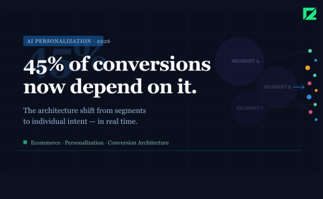
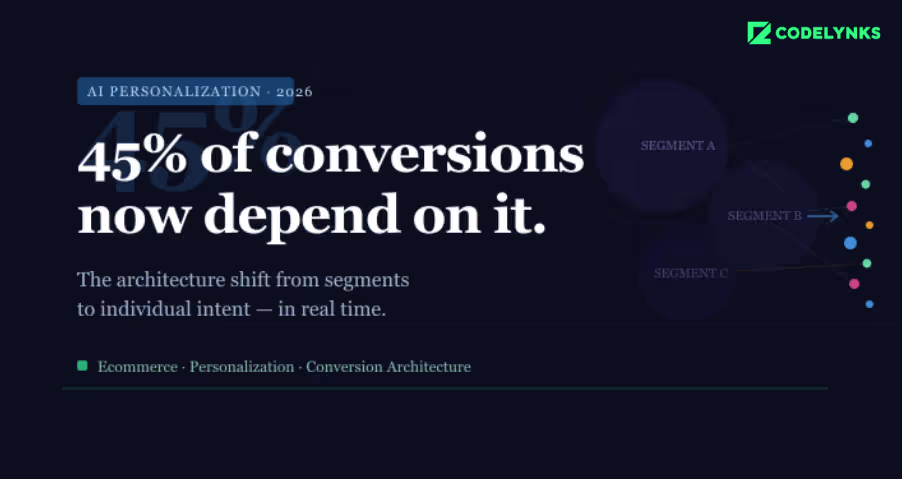
AI personalization in ecommerce has moved from a competitive advantage to a baseline expectation. In 2026, nearly 45% of online conversions are influenced by AI-driven personalization, according to industry analysis.
Most e-commerce product recommendation engines were built on the same premise: group customers into segments and serve each segment a curated experience. Segment-based personalization drove meaningful gains for a decade. In 2026, the data says it is no longer enough.
This post covers what that shift requires architecturally, where most implementations fall short, and how to evaluate whether your current setup can support genuine individual-level personalization. AI personalization in ecommerce now relies on real-time session data instead of static segmentation.
Why AI Personalization in Ecommerce Has Shifted to Real-Time
From Segments to Sessions: What Has Changed : Segment-based personalization works like this: a user who has previously bought running shoes gets shown running accessories. A user in the 25-34 age bracket sees a different homepage banner than a user in the 45-54 bracket. The model is built offline, updated periodically, and applied at request time by looking up the user’s segment and returning pre-computed recommendations.
Individual-level personalization in 2026 works differently. The model observes the current session: what the user clicked, how long they hovered, what they added and then removed from the cart, and what they searched for. It updates its representation of that user’s intent in real time and adjusts the experience, not just the recommendations but also the layout, pricing display, and promotional offers, based on that updated intent.
The distinction matters architecturally. Segment lookup is a read from a pre-computed table. Real-time intent modeling is an inference operation, often involving a neural network, that must be completed within 100-200 milliseconds to avoid impacting page load performance.
The Five Architecture Decisions That Determine Personalization Performance
1. Where inference runs: The most common personalization failure mode is latency. The recommendation model runs in a central data center, 80-150 ms from the user, and the network round trip erodes the user experience before a single recommendation is served.
The biggest limitation of traditional systems is their inability to support AI personalization in ecommerce at the individual level.
The 2026 pattern that high-performing retailers are moving toward is edge inference. Lightweight recommendation models, typically distilled versions of larger models, run at CDN edge nodes close to the user. Full model updates happen centrally and are pushed to the edge on a schedule. The trade-off is model size: edge inference works well for session-level features but cannot run models that require full purchase history or complex cross-session signals.
Decision point: if your target inference latency is under 50ms, edge inference is worth the architecture complexity. If 100-150ms is acceptable, central inference with a well-placed CDN layer is simpler and usually sufficient.
2. Feature pipeline design: Personalization models are only as good as their features. The feature pipeline is the component that transforms raw behavioral events (clicks, searches, purchases, and hovers) into the numerical representations the model uses.
The two-pipeline pattern is now standard: a batch pipeline that processes historical data and generates user embeddings updated daily or hourly and a streaming pipeline that processes real-time session events and updates the in-session representation. At inference time, the model combines both. Historical context provides the long-range signal; session context provides the intent adjustment.
The most common implementation mistake is running only the batch pipeline and calling it real-time personalization. Batch embeddings updated daily cannot capture within-session intent changes. A user who arrived to browse shoes but then searched for a gift idea is being shown the wrong product three pages into their session.
3. Catalogue embedding and search indexing: Recommendation systems need to match a user representation to products in a large catalog. Naive systems do this with collaborative filtering on interaction matrices. Modern systems embed both users and products in the same vector space and use approximate nearest neighbor (ANN) search to find relevant products in milliseconds.
This requires a vector database. Pinecone, Weaviate, and pgvector (for teams already on PostgreSQL) are the common choices in 2026. The catalogue embedding needs to be updated whenever product attributes, inventory, or pricing changes. Serving recommendations for out-of-stock products or products at the wrong price is a trust problem that is harder to recover from than a lower conversion rate.
4. A/B testing infrastructure: Personalization cannot be validated without proper experimentation infrastructure. The challenge is that standard A/B testing assumes independent assignment: user A sees variant 1, user B sees variant 2, and the two groups do not interact.
In e-commerce, users interact: a recommendation served to one user can influence what another user sees in social contexts, inventory is shared, and pricing changes affect the whole market. Rigorous personalization A/B testing uses holdout groups rather than split tests, ensuring a percentage of users always receive the baseline experience and measurement is against that holdout rather than against a simultaneous variant.
5. Data governance and consent management: Personalization at this level requires significant behavioral data. In markets with GDPR, DPDP (India’s Digital Personal Data Protection Act, effective from 2025), and CCPA, that data collection requires explicit consent and clear data retention policies.
The architecture implication: the consent state must be a first-class signal in the feature pipeline. A user who has opted out of behavioral tracking should receive a degraded but functional experience, not an error. Consent management platforms need to integrate directly with the event collection layer, not as an afterthought in the front end.
Businesses investing in AI personalization in ecommerce are seeing measurable conversion improvements.
Build vs Buy: The 2026 Decision Framework
Managed personalization platforms like Dynamic Yield, Bloomreach, and Nosto have matured significantly. For retailers below $50 million in annual GMV, a managed platform almost always delivers better ROI than a custom build. The engineering cost of building and maintaining a two-pipeline feature system, a vector database, and edge inference infrastructure is significant.
Above $50 million GMV, the calculus shifts. At that scale, the recommendation model is a competitive differentiator. Managed platforms apply the same algorithms to all their clients. A custom model trained on your specific catalog, customer base, and business logic can outperform a generic one meaningfully, and the data to train it well is available.
A hybrid architecture is also common: a managed platform for standard recommendation placements and custom models for the highest-value surfaces like the homepage, checkout, and post-purchase experience.
What the Conversion Data Actually Measures
The 45% of conversions driven by AI personalization figure comes from measuring purchases that followed a personalized recommendation or personalized layout change. It does not measure counterfactual conversions, purchases that would have happened anyway without personalisation.
Realistic lift from implementing individual-level personalization over segment-based systems ranges from 15 to 30% in conversion rate, depending on catalogue size, traffic volume, and the quality of the baseline. Smaller catalogues see smaller lifts because the recommendation space is constrained. Higher-traffic sites see larger lifts because the models have more data to work with.
Average order value lift from personalization is typically 8-15%. The mechanism is product adjacency: a well-trained model surfaces complementary products that the customer would not have found through browse navigation.
Key Takeaway
AI personalization in e-commerce is no longer about segments—it’s about real-time intent modeling at the session level.
To compete in 2026, your architecture must support the following:
sub-200ms inference
streaming + batch feature pipelines
vector-based product retrieval
consent-aware data systems
Retailers who invest in this shift are seeing 15–30% conversion lifts and measurable revenue impact. Those who don’t are optimizing a model that the market has already outgrown. AI personalization in e-commerce is no longer about segments—it is about real-time intent modeling at the session level.
Need help with AI personalization architecture for your e-commerce platform? Talk to our engineering team at Codelynks. Contact us
Kubernetes clusters are expensive to run and expensive to understand. Most engineering teams know their monthly bill; almost none know which workload, team, or feature is responsible for which portion of it. That information gap is where cloud waste lives.
The FinOps Foundation’s State of FinOps 2026 report documents the gap precisely: 98% of FinOps practitioners are now managing AI and cloud spend together, and pre-deployment cost visibility is the top desired capability across organizations of all sizes. Teams that have built this visibility are cutting their Kubernetes bills by 20 to 40 percent without removing features or downgrading performance.
This guide covers the specific practices, tools, and architecture decisions that make that possible.
Why Kubernetes Costs Are Hard to Manage
Traditional cloud cost allocation works at the service or resource level. Kubernetes adds two layers of abstraction: pods share nodes, and nodes are grouped into clusters. A single node bill might represent traffic from a dozen different applications owned by three different teams.
Without active cost attribution, the bill is opaque. You know you spent $40,000 on compute in March. You do not know that $18,000 of that came from a batch job that runs once a day and could run overnight on Spot instances at one-fifth the cost.
The three root causes of Kubernetes waste:
Overprovisioning: Teams request more CPU and memory than workloads use, because the cost of over-requesting is invisible and the cost of under-requesting is an outage.
Idle capacity: Nodes that stay running overnight and on weekends for workloads that only run during business hours.
Unattributed spend: No namespace-level or label-level cost breakdown means no team feels accountable for their portion of the bill.
Step 1: Get Cost Visibility Before You Optimize:
You cannot optimize what you cannot see. The first step is establishing namespace-level and workload-level cost attribution.
GKE Cost Allocation (Now Generally Available) : Google Kubernetes Engine’s cost allocation feature, which became generally available in 2025, breaks down billing by cluster, namespace, and label, and exports that data to BigQuery. If you are on GKE, this is your starting point. Enable it today.
In your GKE cluster settings, enable the Cost Allocation feature under Networking. Configure a BigQuery export in your billing settings. Within 24 to 48 hours you will have namespace-level cost data you can query directly.
A basic BigQuery query to see cost by namespace:
SELECT namespace, SUM(cost)as total_cost FROM `billing_export.gke_cost_allocation`
For Multi-Cloud or Self-Managed Clusters : Tools like Kubecost, OpenCost (CNCF open-source), and Finout provide namespace and label-level cost attribution across AWS EKS, Azure AKS, and self-managed clusters. Kubecost’s free tier covers a single cluster; the paid tier adds multi-cluster rollup and anomaly detection.
The minimum label taxonomy to enforce across all workloads:
team: the owning engineering team
service: the product or service name
environment: production, staging, development
cost-center: the budget code for chargeback
Step 2: Rightsize Before You Buy More
Most Kubernetes performance problems are attributed to insufficient resources, so teams over-provision. The data consistently shows the opposite: the average Kubernetes cluster runs at 20 to 30 percent CPU utilization and 40 to 60 percent memory utilization under normal load.
Vertical Pod Autoscaler (VPA) for Rightsizing Recommendations : VPA in recommendation mode (not enforcement mode) analyzes actual pod resource usage and recommends right-sized requests and limits without changing anything automatically. Run it for two weeks, review the recommendations, and apply changes manually to critical workloads.
To deploy VPA in recommendation mode for a deployment:
apiVersion: autoscaling.k8s.io/v1
kind: VerticalPodAutoscaler
metadata:
name: my-app-vpa
spec.
targetRef:
apiVersion: "apps/v1"
kind: Deployment
name: my-app
updatePolicy:
updateMode: "Off" # Recommendation only, no automatic changes
Check recommendations after 14 days:
kubectl describe vpa my-app-vpa
Teams that right-size based on VPA recommendations typically reduce their compute requests by 30 to 40 percent while maintaining the same performance profile.
Horizontal Pod Autoscaler (HPA) for Bursty Workloads: If your workloads have predictable traffic patterns (higher during business hours, lower at night), HPA with custom metrics can scale down to minimum replicas during off-peak hours automatically. Combined with cluster autoscaler removing idle nodes, this is the single highest-ROI optimization for most teams.
Step 3: Shift Non-Critical Workloads to Spot or Preemptible Instances
Spot instances (AWS) and Preemptible VMs (GCP) cost 60 to 90 percent less than on-demand instances. They can be terminated with 2 minutes of notice. That constraint rules them out for stateful or latency-critical workloads, but opens significant savings for everything else.
Workloads that are suitable for Spot:
Batch processing jobs
CI/CD pipeline workers
Data transformation and ETL
Non-critical background workers
Development and staging environments
The Kubernetes node pool configuration for Spot on GKE:
Use node selectors or tolerations to schedule appropriate workloads onto the spot pool while keeping production workloads on on-demand nodes.
Step 4: Add AI Spend to Your FinOps Scope
The FinOps Foundation’s 2026 survey found that 98% of FinOps teams are now managing AI spend, making it the fastest-growing cost category under FinOps oversight. If your Kubernetes clusters are running ML inference workloads or AI-adjacent services, those costs need the same attribution and optimization treatment as your application workloads.
Specific controls for AI workloads on Kubernetes:
GPU cost allocation: Tag GPU node pools separately and require workloads to justify GPU requests. GPU nodes cost 3 to 8 times more than equivalent CPU nodes.
Inference scheduling: Batch inference workloads to run during off-peak hours when Spot availability is higher and cost is lower.
Model caching: Cache loaded models in memory rather than loading them on each request. Model load time is pure GPU cost with no output.
Cost per inference: Track cost per model query, not just per pod. This connects infrastructure cost to product usage in a way engineers and product managers can both act on.
Step 5: Implement Chargeback to Create Accountability
The most durable cost control is not a technical optimization. It is making teams financially aware of what they consume.
Chargeback allocates actual cloud costs to the teams or cost centers responsible for them. Showback is the lighter version: teams see their costs but are not charged internally. Both work; chargeback creates stronger behavioral change.
A minimal chargeback implementation:
Export namespace-level cost data weekly to a shared dashboard (BigQuery + Looker Studio, or Kubecost’s cost center report)
Send each team lead a weekly cost summary email for their namespaces
Set budget alerts at 80% and 100% of monthly targets per namespace
Review cost anomalies in your weekly engineering sync, not in a separate FinOps meeting
Teams that see their costs consistently make different infrastructure decisions than teams that do not. The change is not dramatic; it is cumulative. Over six months, awareness alone reduces waste by 10 to 15 percent.
What 30% Cost Reduction Actually Looks Like
Based on implementations across multiple clients, the savings stack roughly as follows:
Rightsizing via VPA recommendations: 15 to 25% reduction in compute spend
Spot/Preemptible for non-critical workloads: 10 to 20% of total cluster cost
HPA + cluster autoscaler for off-peak scaling: 5 to 10% reduction
Chargeback-driven behavioral change: 5 to 15% over six months
The exact number depends on your current state. Teams with no optimization in place and no cost attribution tend to see the largest gains quickly. Teams that are already using autoscaling and have some attribution in place see smaller but still meaningful reductions.
The work is not technically complex. It is operationally consistent. The teams that achieve 30% reductions are the ones that treat infrastructure cost as an engineering metric, not an accounting problem.
Need help building a FinOps practice for your Kubernetes environment? Talk to our engineering team at Codelynks.www.codelynks.com/contact